1. Energy scale and resolution calibration
1.1 HE
Figure 1 shows the detected background spectrum from seven hours of blank sky. The background is dominated by internal activation effects. Prominent background lines due to activation of iodine by cosmic and SAA protons are seen at 31, 56, 67 and 191 keV. These four lines can be used to calibrate the Energy-Channel (EC) relation or energy scale. Background line of 191 keV is also used to monitor the long-term stability of EC relation in-orbit as shown in Figure 2.
The energy resolution for 31keV is used to estimate the energy resolution in orbit.
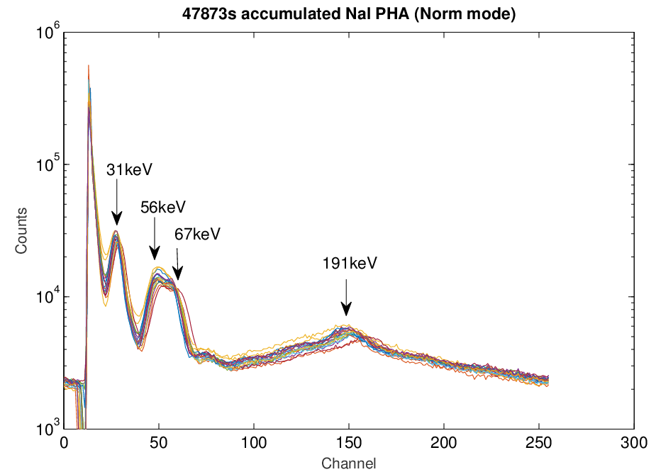
Figure 1: The observed background spectrum detected by 18 PHOSWISH detectors of HE. Background lines due to activation of iodine by cosmic and SAA protons are evident at 31, 56, 67, and 191 keV.
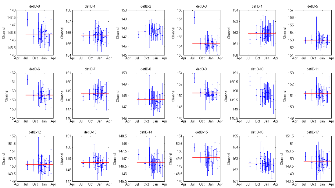
Figure 2: The peak of 191 keV background line can be used to monitor the stability of energy scale for HE detectors.
1.2 ME
The working temperature of ME in-orbit changed between -50℃ and -5℃. In the calibration experiment on ground, we found the Energy-Channel (EC) relation is linear from 11 keV to 30 keV using the spectrum of 241Am source. The slopes and intercepts of E-C relation of all pixels are not a constant at different temperatures as shown in Figure 3. The slopes and intercepts will be achieved from the linear interpolation at two adjacent temperatures for each pixel. In-orbit, the pixels carried 241Am and other pixels which have Ag line are used to verify the change of EC relation on ground. All blank sky data are analyzed to get the peak of Ag line. We found that EC on ground is also suitable. As shown in Figure 4, the mean value of Ag peak is equaled to 22.5 keV, the same with the expected value.


Figure 3: The slope and intercept of Energy-Channel relation for 32 pixels of one ASIC at different temperatures.
The pixels carried 241Am in orbit can also be used to estimate the variation of FWHM. We found that change is very small.
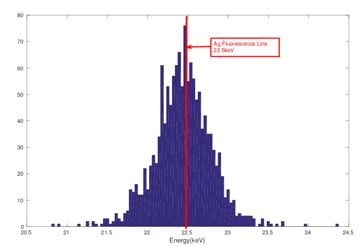
Figure 4: The distribution of Ag line peak for about 1200 pixels
1.3 LE
Ground calibration experiments showed that the linearity of LE was very good, and the slopes and intercepts also differed at different temperatures. The same method for ME was used to obtain the slopes and intercepts at different temperatures.
In-orbit, Cas A was used to verify the change of EC relation. Here, we used the observed spectrum of Chandra to get the model of Cas A and fitted the measured spectrum of LE to check the shape of residual distribution of two instruments. If the shape of the residual distribution is same of the two instruments, we think that it comes from the systematic error of the source model. Otherwise, the EC of LE has changed compared with the result on ground. From the fit result in Figure 5, the EC relation from 1.8 keV to 4 keV has changed, the peaks in this energy range are used to update the EC relation in-orbit.
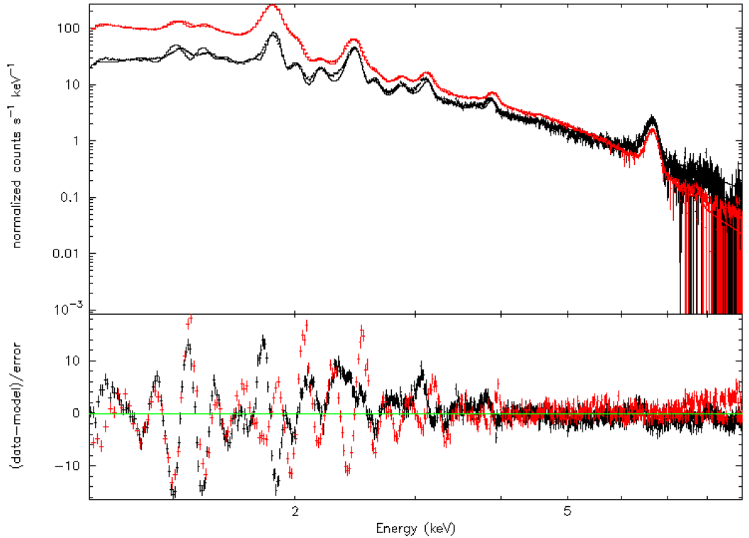
Figure 5: The red dot is the Cas A spectrum measured by Chandra. The black dot is the Cas A spectrum measured by LE. The EC relation from 1.8 keV to 4 keV was different with the on-ground results from the shape distribution of residual distribution.
2. Effective area calibration
2.1 The crab pulsar as a calibration source
The Crab Nebula, with its pulsar has been served as a primary calibration target for many hard X-ray instruments because of its brightness, relative stability, and simple power-law spectrum. The Crab is too bright for most CCD based focusing X-ray instruments because of the pileup effect, but for LE, there are no problems of pileup.
As a collimated telescope, Insight-HXMT has to construct its background model to estimate the background level. There is no on/off observation and it is relatively hard for Insight-HXMT to estimate background because the particle-induced background varies significantly with time and orbit. In order to avoid the influence of background and independently obtain the systematic error of calibration, Crab Pulsar is used to calibrate the effective area of three payloads.
Figure 6 shows the pulse profiles of the Crab pulsar for the entire range of three payloads. The spectrum was generated with the whole pulse and the spectrum of the background is obtained from the phase between 0.6 and 0.8. To acquire the spectral parameter, the spectrum of the Crab pulsar observed by RXTE/PCA and RXTE/HEXTE in the year of 2011(Reference) was calculated with the same method. As shown in Figure 7, the model of the pulsed spectrum can be fitted by LOGPAR(Reference) according to the joint fitting result of two instruments. The fitting parameter alpha is equal to 1.52, beta is equal to 0.139, and norm is equal to 0.448.
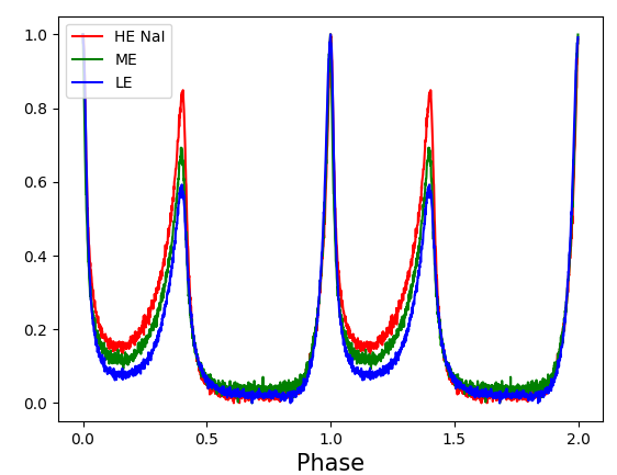
Figure 6: X-ray profiles of Crab Pulsar detected by three payloads of Insight-HXMT. Phase 0 represents the position of the main radio peak. The un-pulsed component is subtracted from phase 0.6 to phase 0.8.
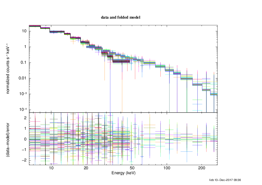
Figure 7: The Crab Pulsar spectrum observed by RXTE/PCA and HXTE in the year of 2011. They jointly determined the model of Crab Pulsar as LOGPAR.
2.2 Results of in-orbit effective areas
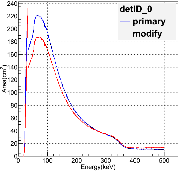
Pure Monte Carlo model of effective area is very difficult to fit the pulsar spectrum well because the absorption and scattering of anticoincidence detectors, non-uniform response of the detectors and so on. Finally, it was decided to use an empirical function to modify the simulated effective areas. The comparisons of the simulated and modified effective areas are shown for three payloads are shown in Figure 8. With the new modified effective areas and fixed the parameters of Crab pulsar, the residual distributions of Crab Pulsar spectrum observed by the three payloads can be found in Figure 9. There is no additional systematics added, 2% will be sufficient for a good fit.

![]()

Figure 8: The comparisons of the primary simulated and modified effective areas. The left one is one NaI(Tl) detector, the middle one is small FOV pixels of ME, and the right one is small FOV CCD236 of LE.
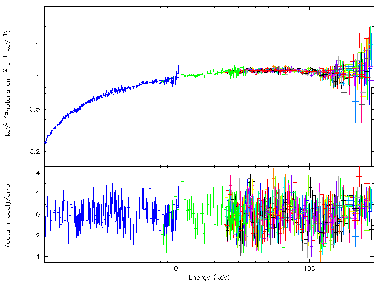
Figure 9: The residual distributions of Crab Pulsar spectrum observed by three payloads of Insight-HXMT with modified effective areas and fixed parameters of Crab Pulsar.
3. Timing calibration
The timing information of Insight was verified through observations of the Crab Pulsar based on the coordinated radio and Fermi-LAT observations. Figure 10 shows the timing residuals of the Pulsar for Insight-HXMT, Radio Telescopes in Xinjiang and Yunnan and Fermi-LAT by TEMPO2. The timing residuals observed from Insight-HXMT are almost the same with the other two instruments. At the end, absolute time accuracy of HXMT is better than 100us from the root-mean-square of timing residual 51 us.
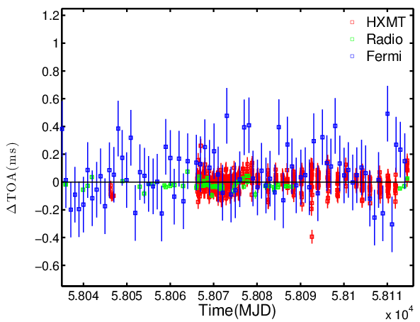
Figure 10: The residuals of TOA of Crab for Radio, Fermi/LAT, and HXMT. The absolute time accuracy of HXMT is better than 100us.